Optimal Mixed Discrete-Continuous Planning for Linear Hybrid Systems

Abstract: Planning in hybrid systems with both discrete and continuous control variables is important for dealing with real-world applications such as extra-planetary exploration and multi-vehicle transportation systems. Meanwhile, generating high-quality solutions given certain hybrid planning specifications is crucial to building high-performance hybrid systems. However, since hybrid planning is challenging in general, most methods use greedy search that is guided by various heuristics, which is neither complete nor optimal and often falls into blind search towards an infinite-action plan. In this paper, we present a hybrid automaton planning formalism and propose an optimal approach that encodes this planning problem as a Mixed Integer Linear Program (MILP) by fixing the action number of automaton runs. We also show an extension of our approach for reasoning over temporally concurrent goals. By leveraging an efficient MILP optimizer, our method is able to generate provably optimal solutions for complex mixed discrete-continuous planning problems within a reasonable time. We use several case studies to demonstrate the extraordinary performance of our hybrid planning method and show that it outperforms a state-of-the-art hybrid planner, Scotty, in both efficiency and solution qualities.

Planning with Linear Hybrid Automata

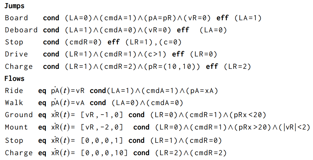
In this work, we use automata to specify our planning problem. A linear hybrid automaton with inputs is a tuple $\mathcal{H} = \langle V = (Q \cup E), q_\texttt{init}, q_\texttt{goal}, J, F \rangle $: (1) $Q = L \cup X$ is the set of state variables. $L$ is the set of discrete state variables, and $X$ is the set of continuous state variables. (2) $E$ is the set of input variables (3) $q_\texttt{init}$ is an initial state, and $q_\texttt{goal}$ is a predicate that represents a set of goal states. (4) $J$ is the set of jumps. A jump is associated with a condition $\textit{cond}$ and an effect $\textit{eff}$. The condition $\textit{cond}$ is a predicate, which is also known as the guard condition or the enabling condition of the jump. An effect $\textit{eff}$ specifies how the value of the state variables changes when the jump occurs. (5) $F$ is the set of flows for the state variables. A flow is associated with a differential equation and a condition. At each time, multiple flows $f \in F$ can be activated and together specify the evolution of the continuous state variables. A valid solution is a valid run of this automaton.

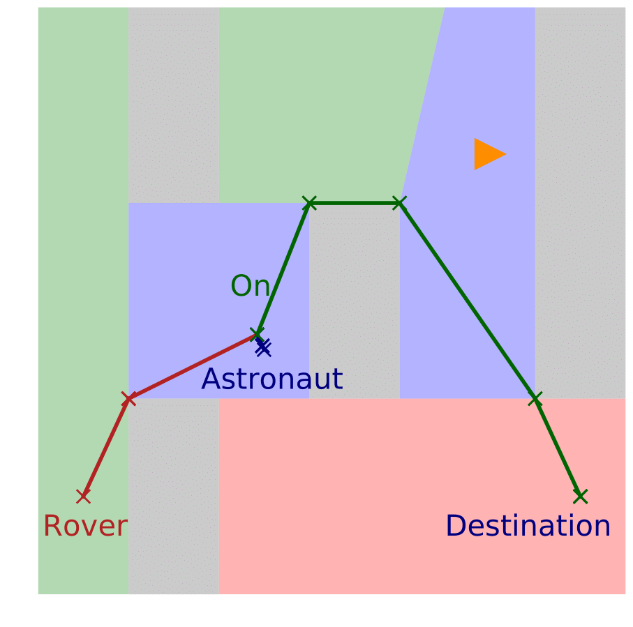
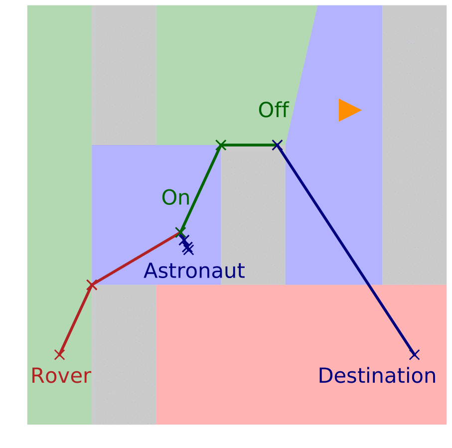
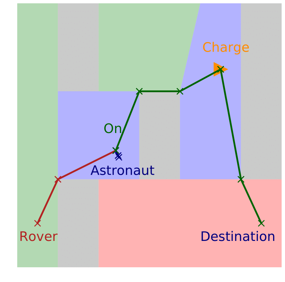
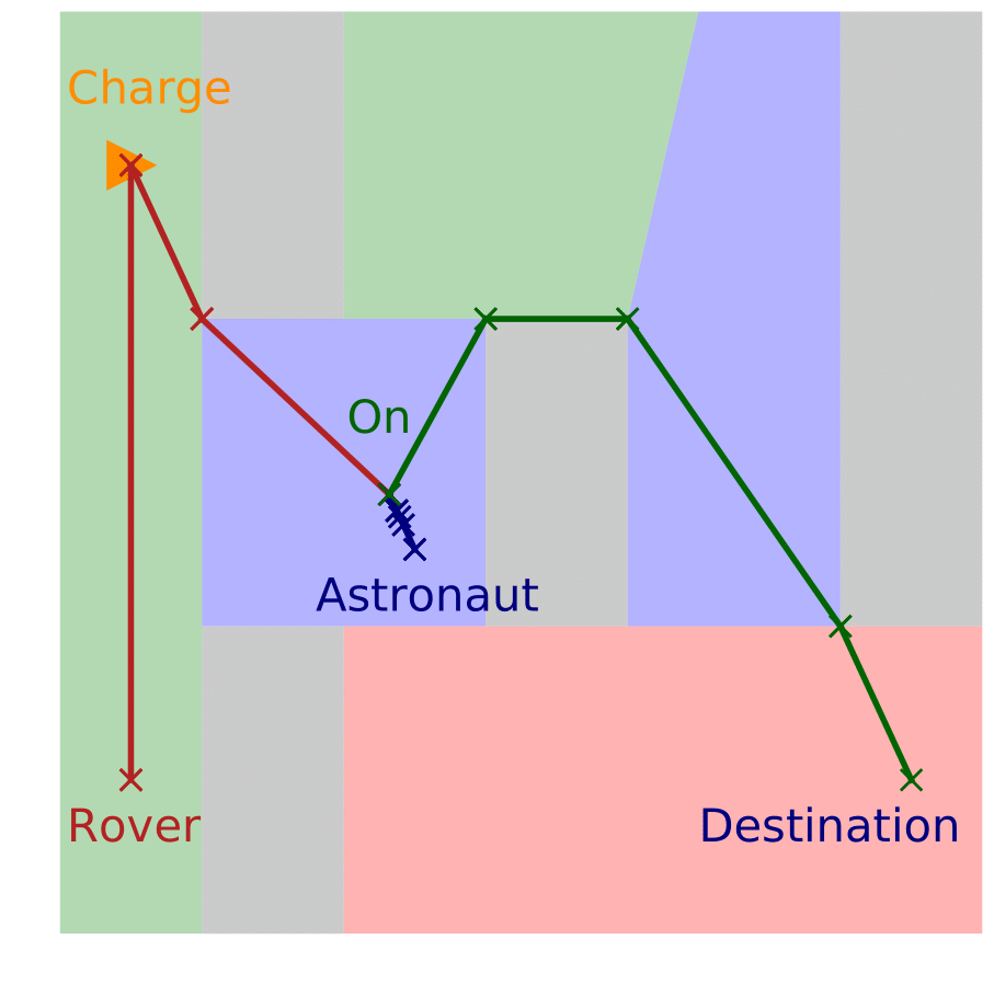
Consider a task where an astronaut should go to an observation location by crossing different terrains (e.g., mountain, ground, and basin) on Mars, and a rover needs to go to the charge station. The astronaut can either walk or take a rover. The moving speed of the rover is much faster than the walking speed of the astronaut. The rover is powered by a battery. This battery can be charged when the rover is stopped in a charge station and should always have the remaining battery outside of the charge station. While the rover and astronaut should not enter the forbidden areas, the rover can move through different terrains with different velocity limits and energy consumption rates. After the rover is manually shut down, it cannot restart within 1 minute. In this mission, plans with shorter makespans are preferred. A high-quality plan is that while the astronaut is moving towards the rover, the rover moves to the charge station for charging, then picks up and delivers the astronaut to the destination, and finally returns to the charge station. As the rover moves much faster than the astronaut, this plan requires much less time than letting the astronaut walk to the destination.

Solving as Mixed Integer Linear Programs

We model the above automata as a MILP and solve by using Gurobi. Our MILP encoding is a mixed integer-linear extension to the linear program encoding of flow tubes with linear dynamics. In this encoding, the elapsed time of each action is modeled as an variable to be adaptive. Thus, this encoding only requires mush less variables than discretizing timeliens with fixed time steps and can support long-horizon planning.

We define a set of variables $\{Q_0, Q_1,.., Q_n\}$ after $a_i$ occurs and right before $a_{i+1}$ occurs. We also have $E_i \in \{E_0,E_1,..,E_{n-1}\}$, corresponding to the values of $E$ when $a_i$ occurs. To represent the actions that happen at each step, we define a set of binary activation variables $\{P_0, P_1,..,P_{n-1}\}$. $P_i$ is the union of $P^J_i$ and $P^F_i = P^{F_0}_i \cup P^{F_1}_i \cup,..,P^{F_K}_i$, which are the activation variables at step $i$ for jumps $J$ and flows $\{F_1, F_2,..,F_K\}$, respectively. Each $p_i^o \in P_i$ corresponds to an operator $o$ (i.e., a jump or a flow) at step $i$. If $p_i^o = 1$, operator $o$ is activated at step $i$; otherwise, $o$ is inactivated. To fully determine the effects of flows, we also specify the cumulative effects of the input variables and the elapsed time. Thus, we define $d_i$ with domain $[0,\infty)$ to represent the elapsed time during step $i$; and real variable $\Delta$ denotes $\int_{0}^{d_i} E_i dt$, the cumulative effects of $E_i$ during step $i$.

The minimizing objective is the total elapsed time. There are four kinds of constraints: (1) the initial and goal states are respected; (2) either a jump or a set of flows are active at each steps. (3) the conditions and effects of activated jumps; and (4) the conditions and effects of activated flows. In this encoding, the implication and conditional activation are expressed by using the Big-M method. And the variable and constraint numbers only increase linear as the variables and operators in the automata increase.

Experimental Results

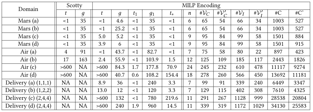
To demonstrate the efficiency and solution qualities of our method, we benchmarked against Scotty on three domains: Mars transportation, air refueling, and truck-and-drone delivery. In addition to dealing with different dynamics under a large number of modes, all these three domains require judiciously coordinating heterogeneous agent teams for cooperation and carefully reasoning over resources to decide necessary recharging or refueling. The experimental results show that our approach can find high-quality solutions for all the problems in seconds and provide optimality proof for most examples, while Scotty fails to solve half of the problems within 600 seconds. Moreover, the makespans of our first solutions returned within $1$ second are already better than those of Scotty, and our final solutions can significantly improve them.

Mars Transportation Domain

The Mars transportation domains involve reasoning over obstacle avoidance and battery consumption under different terrains, such that the astronaut can reach the destination with the help of the rover in the shortest time. We test on four cases: (1) the rover directly picks up and delivers the astronaut to the destination; (2) the rover does not have enough battery for the trip or going to the charge station, and the astronaut has to walk; (3) the rover picks up and delivers the astronaut but has to recharge during the trip; (4) the rover picks up and delivers the astronaut after recharging.

Air Refueling Domain

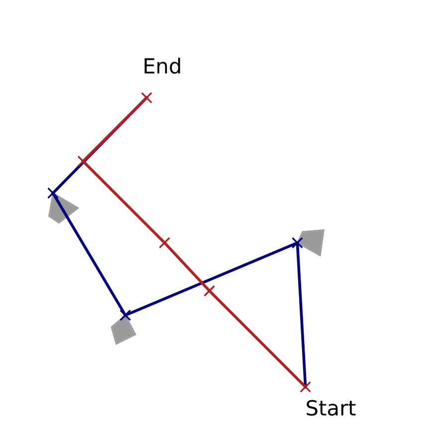
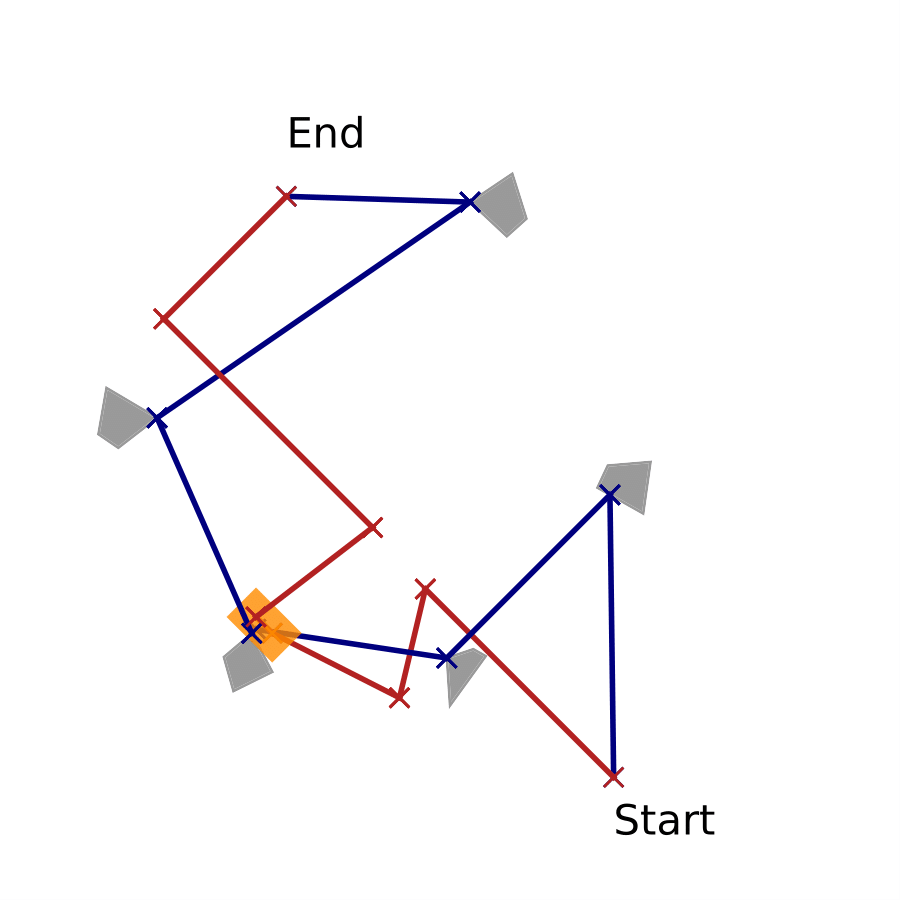
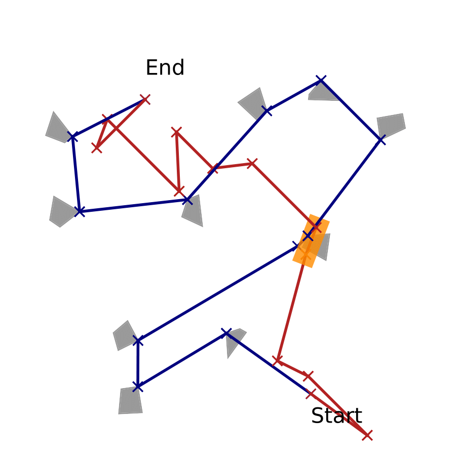
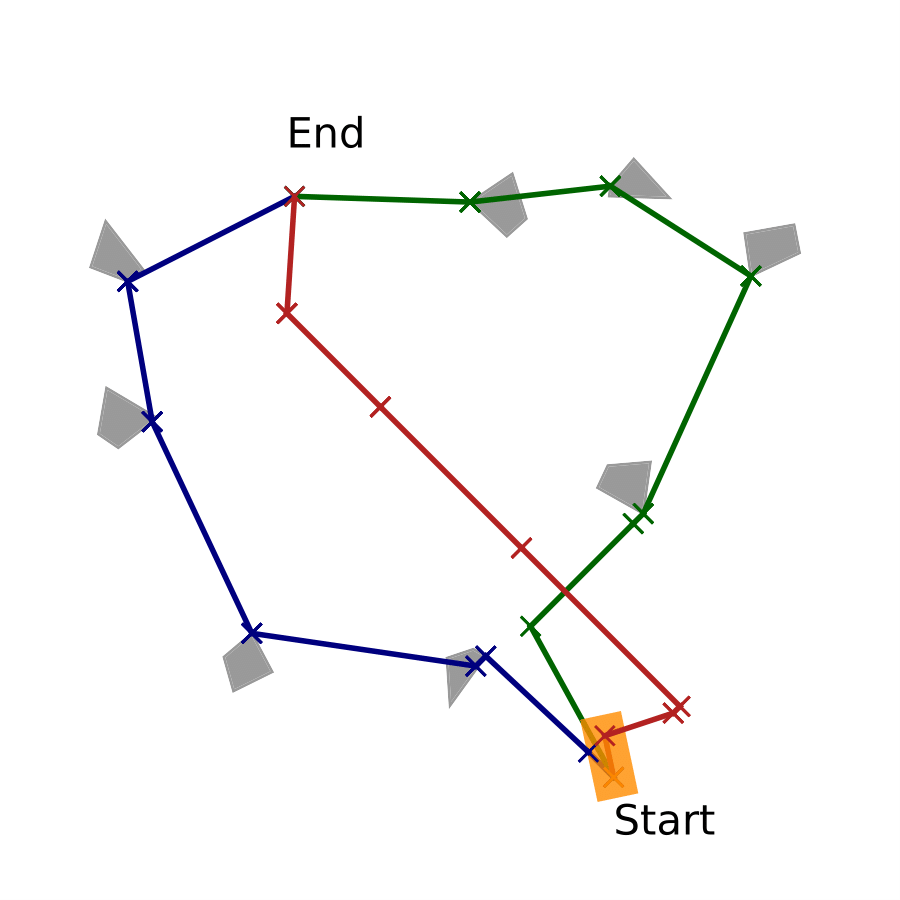
In this domain, autonomous Unmanned Aerial Vehicles (UAVs) need to take pictures of several regions before landing at the destination location. Since a UAV has limited fuel, it needs to refuel in-air from a tanker plane. (1) the UAV takes photos for three regions and does not need refuelingl; (2) the UAV takes photos for four regions and refuels once along the route; (3) the UAV takes photos for ten regions and refuels twice along the route; (4) two UAVs take photos for eight regions along two different routes. While one UAV does not need refueling, the other one refuels once.

Truck-and-Drone Delivery Domain

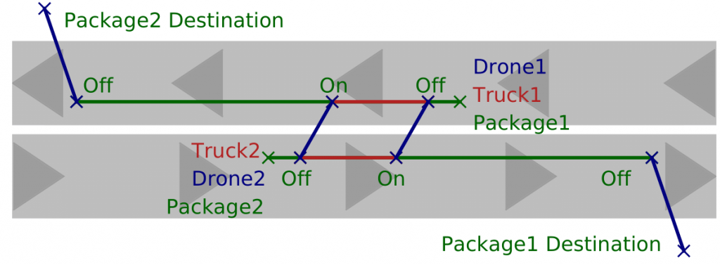
In this domain, we consider a fleet of delivery trucks, each equipped with a couple of drones, and the drone and truck both make deliveries to the customers. While trucks can travel between depots through highways or roads, the drone can fly freely in obstacle-free regions or land on trucks to take a ride. An example between two depots is as follows: the two trucks loaded with packages and drones are driving towards each other on a two-way street. Unfortunately, the package destinations are not on the road ahead, and the trucks cannot turn around. A reasonable plan is that the packages are swapped to the other truck by using the drones to cross the street, and then the truck and drone on the other side continue delivery.