Learning Certified Control using Contraction Metric

Abstract: In this paper, we solve the problem of finding a certified control policy that drives a robot from any given initial state and under any bounded disturbance to the desired reference trajectory, with guarantees on the convergence or bounds on the tracking error. Such a controller is crucial in safe motion planning. We leverage the advanced theory in Control Contraction Metric and design a learning framework based on neural networks to co-synthesize the contraction metric and the controller for control-affine systems. We further provide methods to validate the convergence and bounded error guarantees. We demonstrate the performance of our method using a suite of challenging robotic models, including models with learned dynamics as neural networks. We compare our approach with leading methods using sum-of-squares programming, reinforcement learning, and model predictive control. Results show that our methods indeed can handle a broader class of systems with less tracking error and faster execution speed. Code is available at https://github.com/sundw2014/C3M. The paper is available at https://arxiv.org/abs/2011.12569.

Problem definition

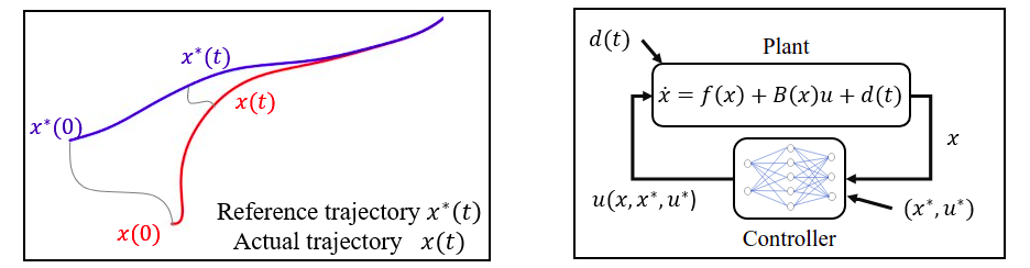
Formally, given a control-affine system $\dot{x} = f(x) + B(x)u$, we want to find a feedback controller $u(\cdot,\cdot,\cdot)$, so that for any reference $(x^*(t), u^*(t))$ solving the ODE, the closed-loop system perturbed by $d$ $$ \dot{x} = f(x(t)) + B(x(t))u(x(t),x^*(t),u^*(t)) + d(t)$$ satisfies that the tracking error $|x(t) – x^*(t)|$ is upper bounded, for all $|d(t)| \leq \epsilon$ and all initial condition $x(0) \in \mathcal{X}$.

Contraction analysis

Contraction analysis can be viewed as a differential version of Lyapunov’s theory. It analyzes the incremental stability by considering the evolution of the distance between two neighboring trajectories of the system. Lyapunov’s theory considers whether the trajectories will finally converge to a point (equilibrium), while contraction theory considers whether all the trajectories converge to a common trajectory. Control contraction metric (CCM) theory extends the analysis to cases with control input, which enables tracking controller synthesis.

Consider a system $\dot{x} = f(x) + B(x) u$, its virtual displacement $\delta_x$ between any pair of arbitrarily close neighboring trajectories evolves as $\dot{\delta}_x = A(x, u) \delta_x + B(x) \delta_u$, where $A(x,u) := \frac{\partial f}{\partial x} + \sum_{i=1}^{m}u^i\frac{\partial b_i}{\partial x}$.

We say $M : \mathcal{X} \mapsto \mathbb{S}_n^{\geq 0}$ is a CCM if there exists a controller $u(x,x^*,u^*)$ s.t. $\forall x, x^*, u^* \in \mathcal{X} \times \mathcal{X} \times \mathcal{U}$, $\forall \delta_x \in \mathcal{T}_{x}{\mathcal{X}}$, $$\frac{d}{dt}\left(\delta_x^\intercal M(x) \delta_x\right) \leq -\lambda \delta_x^\intercal M(x) \delta_x,$$ which implies $\|\delta_x\|_M := \sqrt{\delta_x^\intercal M(x) \delta_x}$ converges to zero exponentially at rate $\lambda$. Such a closed-loop system is referred to be contracting (under metric $M$), which implies good tracking performance.

$$\frac{d}{dt}\left(\delta_x^\intercal M(x) \delta_x\right) \leq -\lambda \delta_x^\intercal M(x) \delta_x,\, \forall \delta_x,\, \forall x,x^*,u^*,$$ $$\dot{\delta}_x = A(x, u) \delta_x + B(x) \delta_u,$$ is equivalent to $\forall x,x^*,u^*$, $$\dot{M} + \mathtt{sym}\left(M(A+BK)\right) + 2 \lambda M \preceq 0,~~~~~(*)$$ where $K := \frac{\partial u}{\partial x}$ and $\mathtt{sym}\left(A\right) = A + A^\intercal$.

Learning a controller with a controller

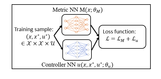
The learning framework.

The loss function is designed as follows.

$$\mathcal{L}_{M,u} (\theta_M, \theta_u) := \mathop{\mathbb{E}}_{x,x^*,u^* \sim \mathtt{Unif}}\left[L_{NSD}\left(\dot{M} + \mathtt{sym}\left(M(A+BK)\right) + 2 \lambda M\right)\right],$$ where $L_{NSD} : \mathbb{R}^{n \times n} \mapsto \mathbb{R}_{\geq}$ and $L_{NSD}(A) = 0$ iff. matrix $A$ is negative semi-definite.

Obviously, by assuming the LHS of $(*)$ is continuous, $$\mathcal{L}_{M,u} = 0~~~\Longleftrightarrow~~~~~(*)\text{ holds } \forall x,x^*,u^* \in \mathcal{X} \times \mathcal{X} \times \mathcal{U}.$$

Experimental results

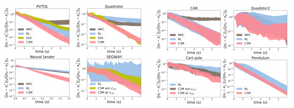
The above figures show the tracking error of the proposed method and several others. The proposed method outperforms all the others. It is worth mentioning that $\texttt{Quadrotor}$ is a $9$-dimensional system, and part of the dynamics of $\texttt{Neural Lander}$ is represented as an NN.